Tutorials
Harmonic and Anharmonic Thermochemistry
This tutorial explains step by step how to use the panther package to calculate the thermodynamic functions of molecules and solids making use of the standard harmonic vibrational analysis and anharmonic vibrations in the independent mode approximation as explained in detail in references [1], [2], [3].
For each step some of the data will be explicitly printed to illustrate the underlying data structures, however in production runs such level of verbosity is not necessary.
The methanol molecule will be used as and example and VASP code will be used to perform the calculations, however since panther is interfaced with ASE any of the supported calculators can be used instead with appropriate modifications.
Structure relaxation
First of all the molecule needs to be relaxed and it is recommended to
converge the forces below 1.0e-5 eV/A. Here the initial structure is
read from the methanol.xyz file and the structure relaxation is performed using
the LBFGS method implemented in ASE instead of the internal VASP optimizers.
import ase.io
from ase.calculators.vasp import Vasp
from ase.optimizers import LBFGS

meoh = ase.io.read('methanol.xyz')

calc = Vasp(
        prec='Accurate',
        gga='PE',
        lreal=False,
        ediff=1.0e-8,
        encut=600.0,
        nelmin=5,
        nsw=1,
        nelm=100,
        ediffg=-0.001,
        ismear=0,
        ibrion=-1,
        nfree=2,
        isym=0,
        lvdw=True,
        lcharg=False,
        lwave=False,
        istart=0,
        npar=2,
        ialgo=48,
        lplane=True,
        ispin=1,
)

meoh.set_calculator(calc)

optimizer = LBFGS(meoh, trajectory='relaxed.traj',
                  restart='lbfgs.pkl', logfile='optimizer.log')

optimizer.run(fmax=0.00001)
Hessian matrix
Having optimized the structure we will also need the hessian matrix. We will use internal VASP mode (IBRION=5) to generate the hessian using cartesian coordinate displacements, therefore we need to update the calculator’s parameters. After the hessian is calculated it is read from the OUTCAR symmetrized, converted to atomic units and saved as a numpy array for convenience
from panther.io import read_vasp_hessian

# adjust the calcualtor argument for hessian calculation
calc.set(ibrion=5, potim=0.02)

calc.calculate(meoh)

hessian = read_vasp_hessian('OUTCAR', symmetrize=True, convert2au=True, negative=True)
np.save('hessian', hessian)
Harmonic vibrations and thermochemistry
We can now use the hessian to calculate thermochemical functions in the harmonic oscillator approximation, starting by calcualting the frequencies and normal modes
from panther.vibrations import harmonic_vibrational_analysis

frequencies, normal_modes = harmonic_vibrational_analysis(hessian, meoh,
            proj_translations=True, proj_rotations=True, ascomplex=False)
The resulting frequencies are in atomic units and need to be
converted to Joules and passed to
Thermochemistry to
calculate thermochemical functions
from scipy.constants import value, Planck
from panther.thermochemistry import Thermochemistry

vibenergies = Planck * frequencies.real * value('hartree-hertz relationship')
vibenergies = vibenergies[vibenergies > 0.0]

thermo = Thermochemistry(vibenergies, meoh, phase='gas', pointgroup='Cs')
thermo.summary(T=273.15, p=0.1)
================ THERMOCHEMISTRY =================

   @ T = 273.15 K  p =   0.10 MPa

--------------------------------------------------
Partition functions:
ln q                     :          23.802
    ln q_translational   :          15.574
    ln q_rotational      :           7.949
    ln q_vibrational     :           0.280
--------------------------------------------------
Enthalpy (H)             :         140.014  kJ/mol
    H translational      :           3.407  kJ/mol
    H rotational         :           3.407  kJ/mol
    H vibrational        :         130.930  kJ/mol
        @ 0 K (ZPVE)     :         129.733  kJ/mol
        @ 273.15 K       :           1.197  kJ/mol
        pV               :           2.271  kJ/mol
--------------------------------------------------------------------------
                                                               *T
Entropy (S)              :           0.2355 kJ/mol*K        64.3395 kJ/mol
    S translational      :           0.1503 kJ/mol*K        41.0476 kJ/mol
    S rotational         :           0.0786 kJ/mol*K        21.4591 kJ/mol
    S vibrational        :           0.0067 kJ/mol*K         1.8328 kJ/mol
--------------------------------------------------------------------------
U - T*S                  :          75.6749 kJ/mol
--------------------------------------------------
Electronic energy        :       -2918.9516 kJ/mol
Normal Mode Relaxation
In some cases it is advantegeous to refine the structure using displacements
along normal modes of vibrations, such a functionality is provided through
the NormalModeBFGS which
is based on the
Optimizer
class from the ASE pakckage. The method requires an initial guess for the hessian
matrix for which we’ll reuse the hessian calculated in one of the previous
steps, however in this case the hessian should be in eV/Angstrom^2 units,
therefore it needs to be converted.
from panther.nmrelaxation import NormalModeBFGS

from scipy.constants import angstrom, value

ang2bohr = angstrom / value('atomic unit of length')
ev2hartree = value('electron volt-hartree relationship')

hessian = hessian * (ang2bohr**2) /ev2hartree

# create the optimizer
optimizer = NormalModeBFGS(meoh, 'gas', hessian, logfile='optimizer.log',
                           trajectory='relaxed.traj', proj_translations=True,
                           proj_rotations=True)

# start the relaxation
optimizer.run(fmax=0.001)
Anharmonic Thermochemistry
Internal coordinate displacements
With frequencies and normal modes we can further generate a
grid of displacements along each normal mode using internal coordinates to
improve the sampling of the potential energy surface. This is done using the
calculate_displacements
function. The function returns a nested OrderedDict
of structures as ase.Atoms objects with mode number and displacement sample number as keys.
For example if npoints=4 is given as an argument there will be 8 structures
per mode labeled with numbers 1, 2, 3, 4, -1, -2, -3, -4 signifying the direction
and the magnitude of the displacement.
from panther.displacements import calculate_displacements

images, modeinfo = calculate_displacements(meoh, hessian, frequencies, normal_modes, npoints=4)

print(modeinfo.to_string())

           HOfreq  effective_mass displacement is_stretch vibration     P_stretch        P_bend     P_torsion  P_longrange
mode
0     3748.362703     1944.298846      3.05268       True      True  1.000538e+00  9.633947e-07  3.581071e-08          0.0
1     3033.988514     2003.111476      3.39309       True      True  1.000487e+00  1.444002e-03  1.358614e-08          0.0
2     2956.839029     2015.939983      3.43707       True      True  1.000163e+00  2.112104e-03  0.000000e+00          0.0
3     2897.901987     1886.235715      3.47185       True      True  1.002597e+00  4.553844e-05  0.000000e+00          0.0
4     1445.646111     1896.588719      2.45777      False      True  2.423247e-04  8.382427e-01  1.620089e-01          0.0
5     1430.743791     1910.050531      2.47054      False      True  5.828069e-07  7.696362e-01  2.314594e-01          0.0
6     1413.372913     2064.662087      2.48567      False      True  1.101886e-05  1.013066e+00  1.246737e-02          0.0
7     1320.779390     2344.971044      2.57133      False      True  2.648486e-03  8.819130e-01  1.163030e-01          0.0
8     1122.078049     2310.188376      2.78972      False      True  8.856000e-04  8.562025e-01  1.423684e-01          0.0
9     1043.856152     2998.235955      2.89236      False      True  4.590826e-01  4.698373e-01  7.957428e-02          0.0
10     999.428001     4154.928137      2.95595      False      True  5.647864e-01  3.944914e-01  4.924659e-02          0.0
11     276.606858     1950.430919      5.61876      False      True  5.101834e-06  1.465507e-04  1.002540e+00          0.0
12       0.000000     8792.819312          inf      False     False           NaN           inf           NaN          0.0
13       0.000000     4750.377947          inf       True     False           inf           NaN           NaN          0.0
14       0.000000     6312.514911          inf       True     False           inf           NaN           NaN          0.0
15       0.000000     5243.620927          inf       True     False           inf           NaN           NaN          0.0
16       0.000000     2177.259022          inf      False     False           NaN           inf           NaN          0.0
17       0.000000     8532.108968          inf       True     False           inf           NaN           NaN          0.0
The function also returns modeinfo DataFrame with additional characteristics
of the mode such as displacement, is_stretch and effective_mass and
components of the vibrational population analysis.
Calculating energies for the displaced structures
Per each displaced structure we can calculate the energy, in this example using the VASP calculator again in the single point calculation mode
from panther.pes import calculate_energies

# set the calculator in single point mode
calc.set(ibrion=-1)

energies = calculate_energies(images, calc, modes='all')
This will return a DataFrame with npoints * 2 energies per mode.
The energies are missing the equilibrium structure energy which can be
easily set through
energies['E_0'] = meoh.get_potential_energy()

print(energies.to_string())

         E_-4       E_-3       E_-2       E_-1        E_0        E_1        E_2        E_3        E_4
0  -29.838210 -29.999174 -30.129845 -30.219158 -30.252801 -30.212111 -30.072575 -29.801815 -29.357050
1  -29.887274 -30.033740 -30.148793 -30.224943 -30.252801 -30.220603 -30.113614 -29.913317 -29.596341
2  -29.765209 -29.983697 -30.134831 -30.223555 -30.252801 -30.223573 -30.135003 -29.984312 -29.766713
3  -29.880739 -30.032824 -30.149891 -30.225671 -30.252801 -30.222657 -30.125177 -29.948635 -29.679366
4  -30.194580 -30.220226 -30.238397 -30.249217 -30.252801 -30.249248 -30.238656 -30.221115 -30.196709
5  -30.196107 -30.220941 -30.238652 -30.249266 -30.252801 -30.249268 -30.238667 -30.220985 -30.196211
6  -30.199391 -30.222460 -30.239171 -30.249354 -30.252801 -30.249264 -30.238446 -30.219995 -30.193484
7  -30.202508 -30.224242 -30.239987 -30.249567 -30.252801 -30.249516 -30.239548 -30.222731 -30.198903
8  -30.208386 -30.227840 -30.241715 -30.250030 -30.252801 -30.250030 -30.241714 -30.227847 -30.208412
9  -30.209316 -30.228681 -30.242227 -30.250194 -30.252801 -30.250259 -30.242766 -30.230511 -30.213676
10 -30.210619 -30.229477 -30.242607 -30.250294 -30.252801 -30.250378 -30.243261 -30.231673 -30.215822
11 -30.241961 -30.246534 -30.249960 -30.252081 -30.252801 -30.252072 -30.249935 -30.246486 -30.241889
Calculating the frequencies
Frequencies can now be calculated using the finite difference method implemented in
panther.pes.differentiate() function and appended as a frequency column
to the modeinfo. The returned vibs matrix contains four columns corresponding
to derivatives calculated with the central formula using 2, 4, 6 and 8 points
from panther.pes import differentiate
from scipy.constants import value

dsp = modeinfo.loc[modeinfo['vibration'], 'displacement'].astype(float).values
vibs = differentiate(dsp, energies, order=2)

au2invcm = 0.01 * value('hartree-inverse meter relationship')
np.sqrt(vibs) * au2invcm

array([[ 3757.6949986 ,  3745.36173164,  3745.5117494 ,  3745.51978786],
       [ 3038.75202112,  3032.49074659,  3032.55620542,  3032.56159197],
       [ 2960.0679129 ,  2956.11388526,  2956.13869496,  2956.14205087],
       [ 2900.20373811,  2897.17093192,  2897.18620368,  2897.18888617],
       [ 1446.18374932,  1446.16517443,  1446.1824322 ,  1446.19041632],
       [ 1431.77027217,  1431.68206976,  1431.68116942,  1431.68294377],
       [ 1414.58204596,  1414.17987052,  1414.182009  ,  1414.18039006],
       [ 1321.14267911,  1321.22424463,  1321.24026442,  1321.2470148 ],
       [ 1122.70558461,  1122.64210276,  1122.63752157,  1122.63384929],
       [ 1043.87393741,  1043.78448965,  1043.78296923,  1043.78025961],
       [  999.41759187,   999.30803727,   999.31024481,   999.30971807],
       [  285.06040099,   285.79248818,   285.87505212,   285.9193547 ]])

# assign the frequencies fitted with 8 points to a frequency column
# in the modeinfo
modeinfo.loc[modeinfo['vibration'], 'frequency'] = (np.sqrt(vibs)*au2invcm)[:, 3]
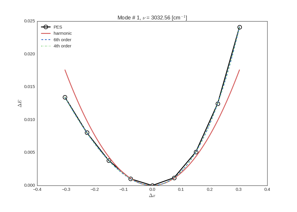
Fitting the potentials
The last this is to fit the potential energy surfaces as 6th and 4th order polynomials
from panther.pes import fit_potentials

# fit the potentials on 6th and 4th order polynomials
c6o, c4o = fit_potentials(modeinfo, energies)
The two DataFrame objects c6o and c4o contain fitted polynomial coefficients for each
mode. We can use the energies and the polynomial coefficients to plot the PES and the fitted
potentials, here as an example, second mode (mode=1 since the modes are indexed from 0) is
plotted
from panther.plotting import plotmode

plotmode(1, energies, modeinfo, c6o, c4o)
Anharmonic frequencies from 1-D Schrodinger Equation
Anharmonic frequencies are calculated first by solving the 1-D Schrodinger equation per mode as exaplained in reference [4] and then those frequencies are used to calculate the thermodynamic functions
from panther.anharmonicity import anharmonic_frequencies, harmonic_df, merge_vibs
from panther.thermochemistry import AnharmonicThermo

anh6o = anharmonic_frequencies(meoh, 273.15, c6o, modeinfo)
anh4o = anharmonic_frequencies(meoh, 273.15, c4o, modeinfo)

harmonicdf = harmonic_df(modeinfo, 273.15)
finaldf = merge_vibs(df6, df4, hdf, verbose=False)

at = AnharmonicThermo(fdf, meoh, phase='gas', pointgroup='Cs')
at.summary(T=273.15, p=0.1)
================ THERMOCHEMISTRY =================

  @ T = 273.15 K  p =   0.10 MPa

--------------------------------------------------
Partition functions:
ln q                     :          23.667
    ln qtranslational    :          15.574
    ln qrotational       :           7.949
    ln qvibrational      :           0.145
--------------------------------------------------
Enthalpy (H)             :         138.890  kJ/mol
    H translational      :           3.407  kJ/mol
    H rotational         :           3.407  kJ/mol
    H vibrational        :         129.806  kJ/mol
        @ 0 K (ZPVE)     :         129.675  kJ/mol
        @ 273.15 K       :           0.131  kJ/mol
        pV               :           2.271  kJ/mol
--------------------------------------------------------------------------
                                                               *T
Entropy (S)              :           0.2375 kJ/mol*K        64.8694 kJ/mol
    S translational      :           0.1503 kJ/mol*K        41.0476 kJ/mol
    S rotational         :           0.0786 kJ/mol*K        21.4591 kJ/mol
    S vibrational        :           0.0086 kJ/mol*K         2.3627 kJ/mol
--------------------------------------------------------------------------
H - T*S                  :          74.0209 kJ/mol
--------------------------------------------------
Electronic energy        :       -2918.9516 kJ/mol
| [1] | Piccini, G., Alessio, M., Sauer, J., Zhi, Y., Liu, Y., Kolvenbach, R., Jentys, A., Lercher, J. A. (2015). Accurate Adsorption Thermodynamics of Small Alkanes in Zeolites. Ab initio Theory and Experiment for H-Chabazite. The Journal of Physical Chemistry C, 119(11), 6128–6137. doi:10.1021/acs.jpcc.5b01739 |
| [2] | Piccini, G., & Sauer, J. (2014). Effect of anharmonicity on adsorption thermodynamics. Journal of Chemical Theory and Computation, 10, 2479–2487. doi:10.1021/ct500291x |
| [3] | Piccini, G., & Sauer, J. (2013). Quantum Chemical Free Energies: Structure Optimization and Vibrational Frequencies in Normal Modes. Journal of Chemical Theory and Computation, 9(11), 5038–5045. doi:10.1021/ct4005504 |
| [4] | Beste, A. (2010). One-dimensional anharmonic oscillator: Quantum versus classical vibrational partition functions. Chemical Physics Letters, 493(1-3), 200–205. doi:10.1016/j.cplett.2010.05.036 |